Project Introduction
Purpose:
Echocardiography is the most commonly used modality for assessing the heart in clinical practice. In an echocardiographic exam, an ultrasound probe samples the heart from different orientations and positions, thereby creating different viewpoints for assessing the cardiac function. The determination of the probe viewpoint forms an essential step in automatic echocardiographic image analysis.
Approach:
In this study, convolutional neural networks are used for the automated identification of 14 different anatomical echocardiographic views (larger than any previous study) in a dataset of 8,732 videos acquired from 374 patients. Differentiable architecture search approach was utilised to design small neural network architectures for rapid inference while maintaining high accuracy. The impact of the image quality and resolution, size of the training dataset, and number of echocardiographic view classes on the efficacy of the models were also investigated.
Results:
In contrast to the deeper classification architectures, the proposed models had significantly lower number of trainable parameters (up to 99.9\% reduction), achieved comparable classification performance (accuracy 88.4-96.0\%, precision 87.8-95.2\%, recall 87.1-95.1\%) and real-time performance with inference time per image of 3.6-12.6ms.
Conclusion:
Compared with the standard classification neural network architectures, the proposed models are faster and achieve comparable classification performance. They also require less training data. Such models can be used for real-time detection of the standard views.
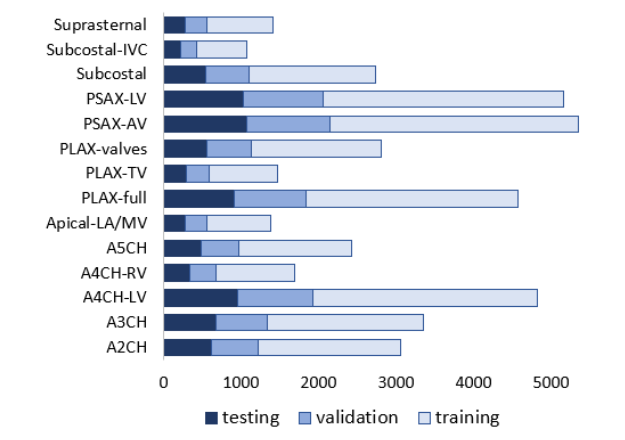
Fig. 1 Distribution of data in the training, validation and test dataset; values show the number of frames in a given class
Dataset
A random sample of 374 echocardiographic examinations of different patients and performed between 2010 and 2020 was extracted from Imperial College Healthcare NHS Trust’s echocardiogram database. The acquisition of the images was performed by experienced echocardiographers and according to standard protocols, using ultrasound equipment from GE and Philips manufacturers.
Ethical approval was obtained from the Health Regulatory Agency (Integrated Research Application System identifier 243023). Only studies with full patient demographic data and without intravenous contrast administration were included. Automated anonymization was performed to remove all patient-identifiable information.
The videos were annotated manually by an expert cardiologist (JPH), categorising each video into one of 14 classes. Videos thought to show no identifiable echocardiographic features, or which depicted more than one view, were excluded. Altogether, this resulted in 9,098 echocardiographic videos. Of these, 8,732 (96.0\%) videos could be classified as one of the 14 views by the human expert. The remaining 366 videos were not classifiable as a single view, either because the view changed during the video loop, or because the images were completely unrecognisable. The cardiologist's annotations of the videos were used as the ground truth for all constituent frames of that video.
DICOM-formatted videos of varying image sizes (480*640, 600*800, and 768*1024 pixels)} were then split into constituent frames, and three frames were randomly selected from each video to represent arbitrary stages of the heart cycle, resulting in 41,321 images. The dataset was then randomly split into training (24791 images), validation (8265 images), and testing (8265 images) sub-datasets in a 60:20:20 ratio. Each sub-datasets contained frames from separate echo studies to maintain sample independence.
The relative distribution of echo view classes labelled by the expert cardiologist is displayed in figure and indicates an imbalanced dataset, with a ratio of 3\% (Subcostal-IVC view as the least represented class) to 13\% (PSAX-AV view as the dominant view).
Network Architecture
DARTS Method:
DARTS method consists of two stages: architecture search and architecture evaluation.
Given the input images, it first embarks on an architecture search to explore for a computation cell (a small unit of convolutional layers) as the building block of the neural network architecture.
Figure 2 provides an overview of the DARTS network architecture.
After the architecture search phase is complete and the optimal cell is obtained based on its validation performance, the final architecture could be formed from one cell or a sequential stack of cells. The weights of the optimal cell learned during the search stage are then discarded, and are initialized randomly for retraining the generated neural network model from scratch.
A cell, shown in figure 2, is an ordered sequence of several nodes in which one or multiple edges meet. Each node C(i) represents a feature map in convolutional networks. Each edge (i,j) is associated with some operation O(i,j), transforming the node C(i) to C(j) . This could be a combination of several operations, such as convolution, max-pooling, and ReLU. Each intermediate node C(i) is computed based on all of its predecessors. Instead of applying a single operation (e.g., 5 × 5 convolution), and evaluating all possible operations independently (each trained from scratch), DARTS places all candidate operations on each edge (e.g., 5 × 5 convolution, 3 × 3 convolution, and max-pooling represented in figure to the right. red, blue, and green lines, respectively). This allows sharing and training their weights in a single process. The task of learning the optimal cell is effectively finding the optimal placement of operations at the edges. The actual operation at each edge is then a linear combination of all candidate operations O(i,j), weighted by the softmax output of the architecture parameters α(i,j).
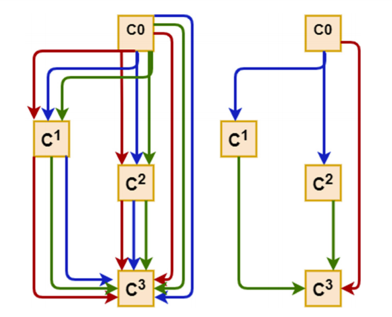
Fig. 2 Schematic of a DARTS cell.
Implementation:
PyTorch was used to implement the models. For the computationally intensive stage of architecture search, a GPU server equipped with 4 NVIDIA TITAN RTX GPUs with 64 GB of memory was rented.
For the subsequent training of the searched networks and also the standard models, the utilized GPU was an Nvidia QUADRO M5000 with 8 GB of memory, representing a more widely accessible hardware for real-time applications. Inference time (latency time for classifying each image) was also estimated with the trained models running on the GPU. To this end, a total of 100 images were processed in a loop, and the average time was recorded.
All training/prediction computations were carried using identical hardware and software resources, allowing for a fair comparison of computational time-efficiency between all network models investigated in this study. The number of trainable parameters in the model, as well as the training time per epoch was also recorded for all CNN networks.
Models Training Parameters
Training occurred subsequently, using annotations provided by the expert cardiologist. It was carried out independently for each of the four different image sizes of 32 × 32, 64 × 64, 96 × 96, and 128 × 128 pixels. Identical training, validation, and testing datasets were used in all network models. The validation dataset was used for early stopping to avoid redundant training and overfitting. Each model was trained until the validation loss plateaued. The test dataset was used for the performance assessment of the final trained models. The DARTS models were kept blind to the test dataset during the stage of architecture search.
Adam optimizer with a learning rate of 10−4 and a maximum number of 800 epochs was used for training the models. The cross-entropy loss was used as the networks objective function. For training the DARTS model, a learning rate of 0.1 deemed to be a better compromise between speed of learning and precision of result and was therefore used. A batch size of 64 or the maximum which could be fitted on the GPU (if <64) was employed.
The dataset is fairly imbalanced with unequal distribution of different echo views. To prevent potential biases towards more dominant classes, we used online batch selection where the equal number of samples from each view were randomly drawn (by over-sampling of underrepresented classes). This led to training on a balanced dataset representing all classes in every epoch. An epoch was still defined as the number of iterations required for the network to meet all images in the training dataset.
Evaluation metrics
Several metrics were employed to evaluate the performance of the investigated models in this study. Overall accuracy was calculated as the number of correctly classified images as a fraction of the total number of images.
Macro average precision and recall (average overall views of perview measures) were also computed.
F1 score was calculated as the harmonic mean of the precision and recall. Since this study is a multi-class problem, F1 score was the weighted average, where the weight of each class was the number of samples from that class..
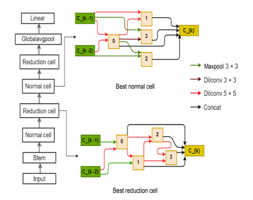
Fig. 3 Optimal normal and reduction cells for the input image size of 128 × 128 pixels
2. View Classification:
Results for five different network topologies and different image sizes are provided in Table 1.
Despite having significantly fewer trainable parameters, the two DARTS models showed competitive results when compared with the standard classification architectures (i.e., VGG16,
ResNet18, and DenseNet201).
The 2-cell-DARTS model, with only ∼0.5-m trainable parameters, achieves the best accuracy (93% to 96%), precision (92.5% to 95.2%), and recall (92.3% to
95.1%) among all networks and across all input image resolutions. Deeper standard neural networks, if employed for echo view detection, would therefore be significantly redundant, with up
to 99% redundancy in trainable parameters.
On the other hand, while maintaining a comparable accuracy to standard network topologies, the 1-cell-DARTS model has ≤0.09 m trainable parameters and the lowest inference time amongst all models and across different image resolutions (range 3.6 to 7.2 ms).
This would allow processing about 140 to 280 frames per second, thus making real-time echo view classification feasible. Compared with manual decision making, this is a significant speedup. Although the identification of the echo view by human operators is almost instantaneous (at least for easy cases), the average time for the overall process of displaying/identifying/recording the echo view takes several seconds.
Having fewer trainable parameters, both DARTS models also exhibit faster convergence and shorter training time per epoch than standard deeper network architectures: 157 116 s versus 622 576 s, respectively, for the training dataset we used.
The confusion matrix for the 2-cell-DARTS model and image resolution of 128 × 128 pixels is provided in Fig. 4. The errors appear predominantly clustered between a certain pair of views which represent anatomically adjacent imaging planes. The A5CH view proves to be the hardest one to detect (accuracy of about 80%), as the network is confused between this view and other apical windows.
This is in line with previous observations that the greatest challenge lies in distinguishing between the various apical views.
Interestingly, the two views the model found most difficult to correctly differentiate (A4CHLV versus A5CH, and A2CH versus A3CH) were also the two views on which the two experts disagreed most often.
The A4CH view is in an anatomical continuity with the A5CH view. The difference is whether the scanning plane has been tilted to bring the aortic valve into view, which would make it A5CH. When the valve is only partially in view, or only in view during part of the cardiac cycle, the decision becomes a judgement call and there is room for disagreement.
Similarly, the A3CH view differs from the A2CH view only in a rotation of the probe anticlockwise, again to bring the aortic valve into view
It is also interesting to note that the misclassification is not fully asymmetrical. For instance,
while 42 cases of A5CH images are confused with A4CH-LV, there are only 14 occasions of
A4CH-LV images mistaken for A5CH.
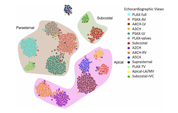
Fig. 5 t-Distributed Stochastic Neighbor Embedding (t-SNE) visualization of 14 echo views from the 2-cell-DARTS model
Figure 6 shows examples of misclassified cases, when the prediction of the 2-cell-DARTS model disagreed with the expert annotation. The error can be explained by the inherent difficulty of deciding, even for cardiologist experts, between views that are similar in appearance to human eyes and are in spatial continuity (case of A4CH/A5CH mix-up), images of poor quality (case of A4CH/PSAX mix-up), or views in which a same view-defining structure may be present (case of PSAX-LV/PSAX/AV mix-up).
3. Impact of Image Resolution, Quality, and Dataset Size
The models seem to exhibit a plateau of accuracy between the two larger image resolutions
of 96 × 96 and 128 × 128 pixels (Fig. 7). On the other hand, for the smaller image size of
32 × 32 pixels, the classification performance seems to suffer across all network models, with
a 2.3% to 5.1% reduction in accuracy relative to the resolution of 96 × 96 pixels.
Shown in Fig. 8’s upper panel, is the class-wise view detection accuracy for various input
image resolutions. Notably, not all echo views are affected similarly using lower image resolutions. The drop in overall performance is therefore predominantly caused by a marked decrease
in detection accuracy of only certain views. For instance, A4CH-RV suffers a sharp reduction of
>10% in prediction accuracy when dealing with images of 32 × 32 pixels.
Figure 8’s lower panel shows the relative confusion matrix, illustrating the improvement
associated with using image resolution of 96 × 96 versus 32 × 32 pixels. Being already a difficult view to detect even in higher resolution images, A5CH will have 47 more cases of misclassified images when using images of 32 × 32 pixels. Overall, apical views seem to suffer the
most from lower resolution images, being mainly misclassified as other apical views.
For instance, the two classes associated with the A4CH will primarily be mistaken for one another.
This is likely because, with a decreased resolution, the details of their distinct features would be
less discernible by the network. Conversely, parasternal views seem to be less affected, and still
detectable in downsampled images. This could be owing to the fact that the relevant features,
on which the model relies for identifying this view, are still present and visible to the model.
Overall, and for almost all echo views, the image size of 96 × 96 pixels appeared to be a good
compromise between classification accuracy and computational costs.
To examine the influence of the size of the training dataset on the model’s performance, we
conducted an additional experiment where we split the training data into sub-datasets with strict
inclusion relationship (i.e., having the current sub-dataset a strict subset of the next sub-dataset),
and ensured all the sub-datasets were consistent (i.e., having the same ratio for each echo view as
in the original training dataset). We then retrained all targeted neural networks on these subdatasets from scratch, and investigated how their accuracy varied with respect to the size of the
dataset used for training the model. The size of the validation and testing datasets, however,
remained unchanged.
Figure 9 shows a drop in the classification accuracy across all models when smaller sizes of
training data are used for training the networks. However, various models are impacted differently. Suffering from redundancy, deeper neural networks require more training data to achieve
similar performances. DenseNet, with the largest number of trainable parameters, appears to be the one which suffers the most, with a 20% reduction in its classification accuracy, when only 8%
of the training dataset is used.
However, the DARTS-based models appear to be relatively less profoundly affected by the
size of the training dataset, where both models demonstrate no more than 8% drop in their prediction accuracy when deprived of the full training dataset. When using fewer than 12,400
images (i.e., 50% of the training dataset), both DARTS-based models exhibit superior performance over the deeper networks.
Additionally, we hypothesized that the more numerous the echo view classes, the more
difficult the task of distinguishing the views for deep learning models, e.g., because of more
chances of misclassifications among classes.
This is potentially the underlying reason for the
inconsistent accuracies (84% to 97%) reported in the literature when classifying between
6 to 12 different view classes. To investigate this premise, we considered cases when only
5 or 7 different echo views were present in the dataset. To this end, rather than reducing the
number of classes by merging several views to create new classes which may not be clinically
very helpful, we were selective in choosing some of the existing classes.
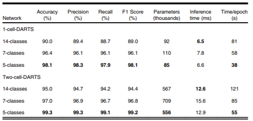
Table 2 The dependence of overall accuracy on the number of echo views
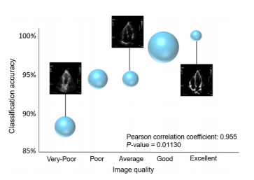
Fig 10 Correlation between the classification accuracy and the image quality
Results and Discussion
1. Architecture Search:
The search took ∼6, 23, 42, and 92 h for image sizes of 32 × 32, 64 × 64, 96 × 96, and 128 × 128 pixels, respectively, on the computing infrastructure described earlier. Figure 3 shows the best convolutional normal and reduction cells obtained for the input image size of 128 × 128 pixels. The retained operations were 3 × 3 and 5 × 5 dilated convolutions, 3 × 3 max-pooling, and skip-connection. Each cell is assumed to have two inputs which are the outputs from the previous and penultimate cells. The output of the cell is defined as the depth-wise concatenation of all nodes in the cell.
Two network architectures were assembled from the optimal cell; “1-cell-DARTS” composed of one cell only,
and “2-cell-DARTS” formed from a sequential stack of two cells.
Addition of more cells to the network architecture did not significantly improve the prediction
accuracy, as reported in the next section, but increased the number of trainable parameters in the
model and thus the inference time for view classification. Therefore, the models with more than
two cells, i.e., architectures with redundancy, were judged as being comparatively inefficient and
thus discarded. Figure 3 (left side) also shows the full architecture for the 2-cell-DARTS model
for the input image size of 128 × 128 pixels.
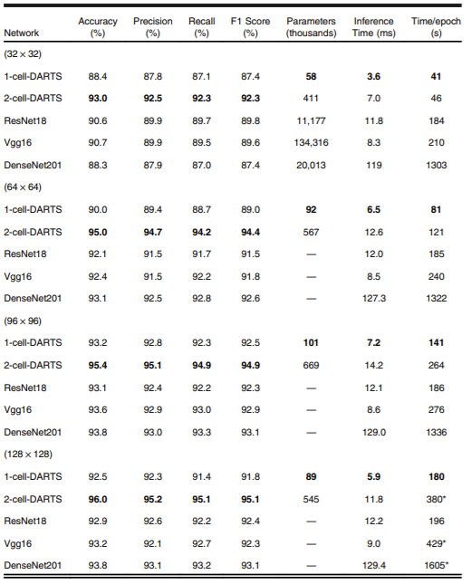
Table 1 Experimental results on the test dataset for input sizes of (32 × 32), (64 × 64), (96 × 96), and (128 × 128) and different network topologies
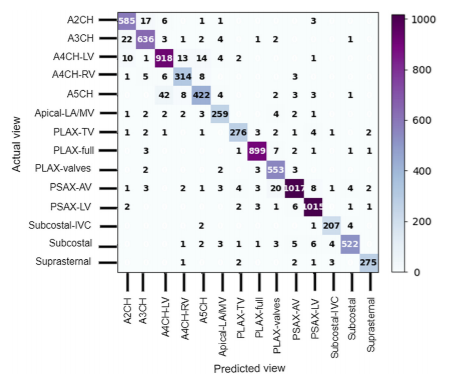
Fig. 4 Confusion matrix for the 2-cell-DARTS model and input image resolution of 128 × 128 pixels.
On the other hand, echo views with distinct characteristics are easier for the model to distinguish. For instance, PLAX-full and Suprasternal seem to have higher rates of correct identification, and the network is confused only on one occasion between these two views. This is also evident on the t-distributed stochastic neighbor embedding (t-SNE) plot in Fig. 5, which displays a planar representation of the internal high-dimensional organization of the 14 trained echo view classes within the network’s final hidden layer (i.e., input data of the fully connected layer). Each point in the t-SNE plot represents an echo image from the test dataset.
Noticeably, not only has the network grouped similar images together (a cluster for each
view, displayed with different color), but it has also grouped similar views together (highlighted
with a unique background color). For instance, it has placed A5CH (blue) next to A4CH (dark
brown), and indeed there is some “interdigitation” of such cases, e.g., for those whose classification between A4CH and A5CH might be debatable. Similarly, at the top right, the network
has discovered that the features of the Subcostal-IVC images (green) are similar to the Subcostal
images (red). This shows that the network can point to relationships and organizational patterns
efficiently.
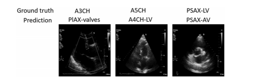
Fig. 6 Three different misclassified examples predicted by the 2-cell-DARTS model for the image resolution of 128 × 128 pixels
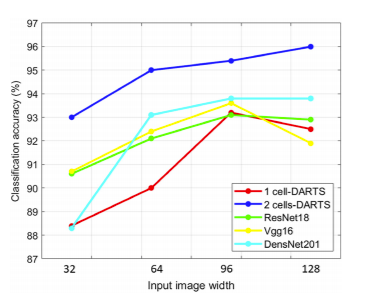
Fig. 7 Comparison of accuracy for different classification models and different image resolutions
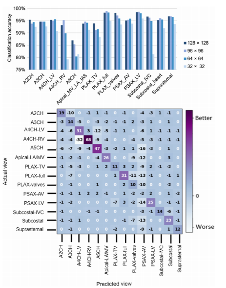
Fig. 8 Accuracy of the 2-cell-DARTS model for various input image resolutions
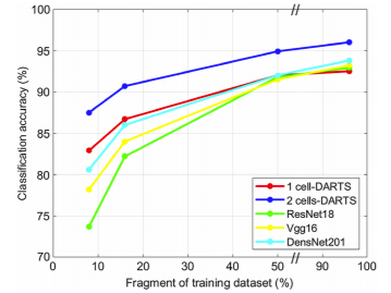
Fig. 9 Comparison of accuracy of different classification models for image size
For each study,we aimed at including views representing anatomically adjacent or similar imaging planes such
as apical windows (thus challenging for the models to distinguish), as well as other echo
windows. The list of echo views included in each study is provided in Table 2.
The results show an increase in the overall prediction accuracy for the two DARTS-based
models, when given the task of detecting fewer echo view classes and despite having relatively
smaller training datasets to learn from. The 1-cell-DARTS model shows 8% improvement in its
performance when the number of echo views is reduced from 14 to 5. The 2-cell-DARTS model
reaches a maximum accuracy of 99.3%, i.e., higher than any previously reported accuracies for
echo view classification. This highlights the fact that for a direct comparison of the classification
accuracy between the models reported in literature, the number of different echo windows
included in the study must be taken into account.
Finally, in order to study the impact of image quality on the classification performance, we
asked a second expert cardiologist to provide an assessment of image quality in the A4CH-LV
views, and assign a quality label to each image where the quality was classified into 5 grades:
very poor, poor, average, good, and excellent. Figure 10 shows the relationship between the
classification accuracy of the 2-cell-DARTS model and the image quality in the test dataset.
The area of the bubbles represents the relative frequency of the images in that quality score
category, with the good category as the dominant grade. This is likely because the image acquisition had been performed mainly by experienced echocardiographers.
The correlation between the classification accuracy and the image quality is evident (p-value
of 0.01). Images labeled as having “excellent” quality, indicated the highest classification accuracy of ∼100%. It is apparent that the discrepancy between the model’s prediction and the expert
annotation is higher in poor quality images. This could potentially be due to the fact that poorly
visible chambers with a low degree of endocardial border delineation could result in some views
being mistaken for other apical windows.