Our team has developed an an optimised-based block matching algorithm to perform speckle tracking iteratively. In this project, a new displacement estimation method is introduced by formulating the tracking as an optimisation problem that jointly penalises intensity disparity and motion discontinuity and is, therefore, more robust to the signal decorrelation when compared with previous approaches. The speckle tracking algorithm combines the BM algorithm with a smoothness constraint for a neighbourhood of kernels. The proposed technique was evaluated using healthy and ischaemic cases.
Dataset
We used a publicly available synthetic echocardiographic dataset with known ground-truth (exact solutions) from several major vendors.
Synthetic ultrasound images from 7 major vendors have been provided: GE, Hitachi-Aloka, Esaote, Philips, Samsung, Siemens, and Toshiba.
To take realistic speckle texture for each vendor, scattering amplitude was sampled from a 2D real clinical recording
ultrasound as a template. Then, an electromechanical cardiac model was used to relocate the scatterers inside the
myocardium and to have a realistic heart motion in the simulated images. Moreover, synthetic probe settings such as
scan depth, focus depth, beam density, etc. were specialised by using the values communicated by each vendor upon
signature of nondisclosure agreements.
Methods
Standard block matching
Classic BM begins by positioning a window on one frame and searching for a pattern with the most similar features
within the dimensions of the placed window in the next frame. A cluster of speckles can be combined into one functional unit which is
called a kernel; each kernel has a unique fingerprint that is determined using a similarity measure and can be
tracked throughout the entire cine loop by the BM algorithm. In the reference frame (first image in Fig. 1, the
current frame or a frame at time t0), the region of interest (blue square) has speckle patterns. In the next frame
(a frame at time t + 1), a broad region of the image is searched for a similar speckle pattern. The location whose
speckle pattern matches best is considered to be the estimated new location of the original kernel, thereby providing an
estimated displacement vector.
This procedure is repeated across the whole of the reference frame, obtaining a displacement map between the two images. Repeating this procedure across the whole image sequence produces a vector field across space and time. In this study, sum of squared differences (SSD) is used as a similarity measure which calculates the difference between the intensity pattern of a grid of pixels (original kernel) in one frame and a set of identically sized kernels in the next frame, to find the best-matched kernel.
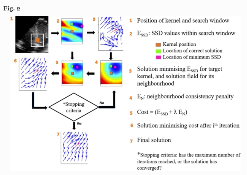
Fig. 2 Flowchart showing the steps involved in solving the proposed optimisation-based tracking algorithm
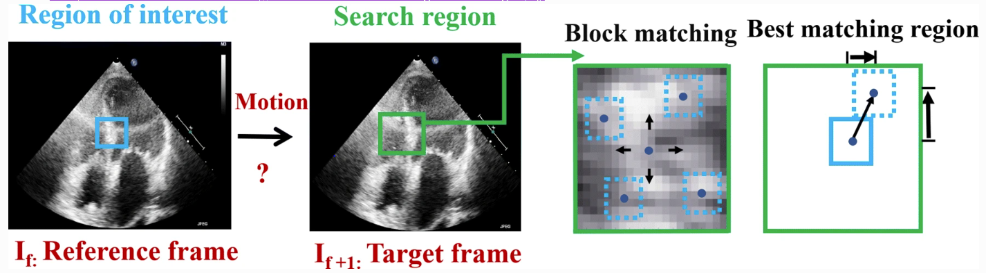
Fig. 1 Speckle tracking using BM where a region in the image (kernel) is selected and sought for in the next image by sequentially trying out different positions, testing the similarity between the kernel and the pattern observed in that position. The position where the similarity between the kernel and the observed pattern is maximal is accepted as the new position of the original kernel
Proposed optimised block matching approach
In this paper, a new displacement estimation method is introduced by formulating the tracking as an optimisation problem that jointly
penalises intensity disparity and motion discontinuity and is, therefore, more robust to the signal decorrelation when compared with
previous approaches. The speckle tracking algorithm combines the BM algorithm with a smoothness constraint for a neighbourhood of kernels,
and minimises the cost function. Fig 2 to the left shows the flow chart of the steps involved in solving the proposed optimisation-based
tracking algorithm.
Tracking parameters
The standard BM was carried out with a kernel size of (11×11) pixels with a spacing of 1 pixel,
providing a dense solution. This kernel size is deemed to be a good compromise for the optimum tracking accuracy.
For the optimised BM approach, the number of iterations was set to 20, which was deemed to be a good compromise between the accuracy and computational run time; a threshold for which the solution was converged and any further update in the displacement vectors were insignificant.
The parameter λ was 0.3, giving more emphasis to the data term versus the regularisation term in the cost function equation.
Larger values of λ tend to heavily regularise the displacement vectors, which would result in an unrealistically uniform vector
field where most of the vectors are aligned. A neighbourhood of (45×45) kernels was included in the iterations for updating the
solution for the central kernel. The tracking accuracy was estimated by comparing the displacement field obtained from the speckle
tracking algorithms and the ground-truth
Results
Displacement vector field
The tracking parameters were similar for all vendors and cases. The algorithm returned a dense displacement
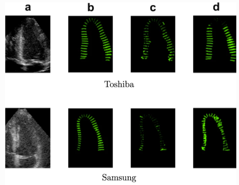
field between pairs of consecutive frames. Figure 3 illustrates an example A4C view from the healthy Siemens
sequence in the rapid ejection phase (peak systole), together with the corresponding ground-truth. a Zoomed view of LV cropped from the original image. b Ground-truth.
c–d Displacement fields obtained from standard BM and optimised BM approach in the rapid ejection phase, respectively.
The computed displacement vector field by the two tracking approaches (standard BM and optimised BM approach)
is also shown. The presence of noise in the results is evident in the standard BM technique, whereas the optimised
BM approach seems to suffer less from this problem.
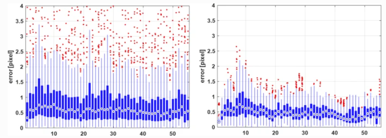
Fig 4: Boxplots of the error for the healthy sequence from Siemens.
Regional and global strain measurements
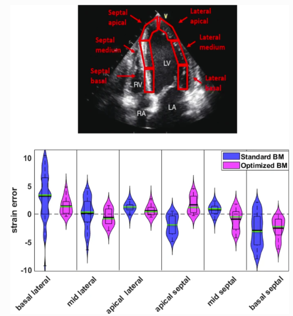
Regional (segmental) longitudinal strain values were calculated from the estimated displacement vector field. Figure 6 displays the violin plots of the regional strain error the difference between the speckle tracked and the ground-truth) for all LV segments, for the same image sequence as shown in Figs. 3 and 4.
Top: an A4C view with the LV myocardium segmentation regions overlaid.
Below: violin plots of the error in the segmental strain measurements for the healthy synthetic sequence from Siemens. The solid black line represents mean, and the green line represents the median; the box signifies the quartiles, and the whiskers represent the 2.5% and 97.5% percentiles
More results and details are in the full paper, the link is in the refereces section.
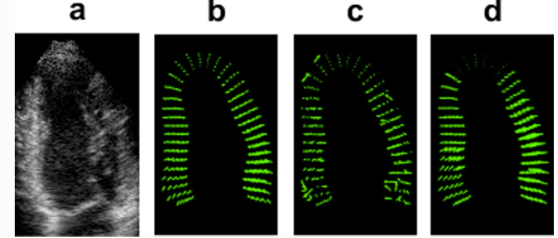
Fig 3: an example A4C view from the healthy Siemens sequence in the rapid ejection phase
Figure 4 shows the distribution of error for the same image sequence, obtained from both tracking methods. The displacement errors across all vendors for their corresponding healthy image sequences are shown in Fig. 5. The error is computed as the magnitude of the difference between the calculated and ground-truth displacement vectors and is provided for standard (left) and proposed (right) tracking methods. The x-axis shows the frame number