Project Introduction
The segmentation of Left Ventricle (LV) is currently carried out manually by the experts, and the automation of this process has proved challenging due to the presence of speckle noise and the inherently poor quality of the ultrasound images. This study aims to evaluate the performance of different state-of-the-art Convolutional Neural Network (CNN) segmentation models to segment the LV endocardium in echocardiography images automatically. Those adopted methods include U-Net, SegNet, and fully convolutional DenseNets (FC-DenseNet). The prediction outputs of the models are used to assess the performance of the CNN models by comparing the automated results against the expert annotations (as the gold standard). Results reveal that the U-Net model outperforms other models by achieving an average Dice coefficient of 0.93 ± 0.04, and Hausdorff distance of 4.52 ± 0.90.
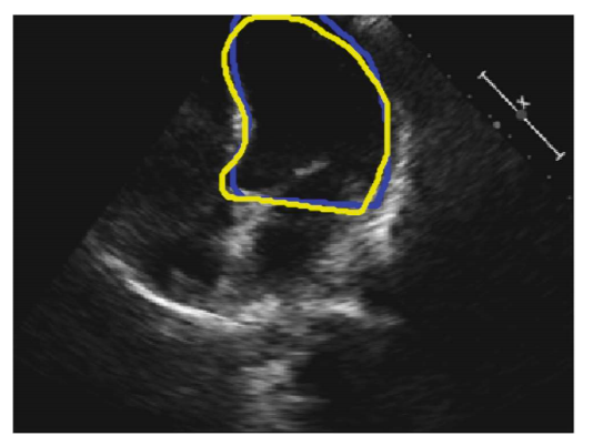
Fig. 1. An example 2D 4-chamber view. The blue and yellow curves represent the annotations by Operator-A and Operator-B, respectively
Dataset
The study population consisted of 61 patients (30 males), with a mean age of 64 ± 11,
who were recruited from patients who had undergone echocardiography with Imperial
College Healthcare NHS Trust. Only patients in sinus rhythm were included. No other
exclusion criteria were applied. The study was approved by the local ethics committee
and written informed consent was obtained.
Each patient underwent standard Transthoracic echocardiography using a commercially available ultrasound machine (Philips iE33, Philips Healthcare, UK), and by experienced echocardiographers. Apical 4-chamber views were obtained in the left lateral
decubitus position as per standard clinical guidelines [3].
All recordings were obtained with a constant image resolution of 480 × 640 pixels.
The operators performing the exam were advised to optimise the images as would typically be done in clinical practice. The acquisition period was 10 s to make sure at least
three cardiac cycles were present in all cine loops. To take into account, the potential
influence of the probe placement (the angle of insonation) on the measurements, the
entire process was conducted three times, with the probe removed from the chest and
then placed back on the chest optimally between each recording. A total of three 10-s
2D cine loops was, therefore, acquired for each patient. The images were stored digitally
for subsequent offline analysis.
To obtain the gold-standard (ground-truth) measurements, one accredited and experienced cardiology expert manually traced the LV borders. Where the operator judged
a beat to be of extremely low quality, the beast was declared invalid, and no annotation was made. We developed a custom-made program which closely replicated the
interface of echo hardware. The expert visually inspected the cine loops by controlled
animation of the loops using arrow keys and manually traced the LV borders using a
trackball for the end-diastolic and end-systolic frames. Three heartbeats (6 manual traces
for end-diastolic and end-systolic frames) were measured within each cine loop. Out of
1098 available frames (6 patients × 3 positions × 3 heartbeats × 2 ED/ES frames), a
total of 992 frames were annotated. To investigate the inter-observer variability, a second operator repeated the LV tracing on 992 frames, blinded to the judgment of the
first operator. A typical 2D 4-chamber view is shown in Fig. 1, where the locations of
manually segmented endocardium by the two operators are highlighted.
Network Architecture
Standard and well-established U-Net neural network architecture was firstly used
since this architecture is applicable to multiple medical image segmentation problems.
The U-Net architecture comprises of three main steps such as down-sampling, upsampling steps and cross-over connections. During the down-sampling stage, the number
of features will increase gradually while during up-sampling stage the original image
resolution will recover. Also, cross-over connection is used by concatenating equally
size feature maps from down-sampling to the up-sampling to recover features that may
be lost during the down-sampling process.
Each down-sampling and up-sampling has five levels, and each level has two convolutional layers with the same number of kernels ranging from 64 to 1024 from top to bottom
correspondingly. All convolutions kernels have a size of (3 × 3). For down-sampling
Max pooling with size (2 × 2) and equal strides was used.
In addition to the U-net, SegNet and FC-DenseNet models were also investigated.
The SegNet model contains an encoder stage, a corresponding decoder stage followed
by a pixel-wise classification layer. In SegNet model, to accomplish non-linear upsampling, the decoder performs pooling indices computed in the max-pooling step of
the corresponding encoder. The number of kernels and kernel size was the same as
the U-Net model.
FC-DenseNet model is a relatively more recent model which consists of a downsampling and up-sampling path made of dense block. The down-sampling path is composed of two Transitions Down (TD) while an up-sampling path is containing two
Transitions Up (TU). Before and after each dense block, there is concatenation and
skip connections (see Fig. 2). The connectivity pattern in the up-sampling is different
from the down-sampling path. In the down-sampling path, the input to a dense block is
concatenated with its output, leading to linear growth of the number of feature maps,
whereas in the up-sampling path, it is not.
All models produce the output with the same spatial size as the input image
(i.e., 320 × 240).
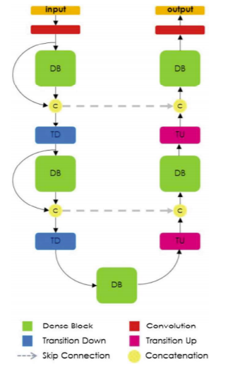
Fig. 2. Diagram of FC-DenseNet architecture for semantic segmentation
Implementation:
Pytorch was used for the implementations [10], where Adam optimiser with 250 epochs and learning rate of 0.00001 were used for training the models.
The network weights are initialised randomly but differ in range depending on the size
of the previous layer.
Negative log-likelihood loss is used as the network’s objective
function. All computations were carried using an Nvidia GeForce GTX 1080 Ti GPU.
All models were trained separately and indecently using the annotations provided
by either of the operators, and following acronyms are used for the sake of simplicity:
GTOA and TOB as ground-truth segmentations provided by Operator-A and Operator-B,
respectively; POA and POB as Predicted LV borders by deep learning models trained
using GTOA and TOB.
Evaluation Measures
The Dice Coefficient (DC), Hausdorff distance (HD), and intersection-over-union (IoU)
also known as the Jaccard index were employed to evaluate the performance and accuracy
of the CNN models in segmenting the LV region. The DC was calculated to measure
the overlapping regions of the Predicted segmentation (P) and the ground truth (GT).
The range of DC is a value between 0 and 1, which 0 indicates there is not any overlap
between two sets of binary segmentation results while 1, indicates complete overlap.
Also, the HD was calculated using the following formula for the contour of segmentation where, d(j, GT, P) is the distance from contour point j in GT to the closest contour
point in P. The number of pixels on the contour of GT and P specified with O and M
respectively.
Moreover, the IoU was calculated image-by-image between the Predicted segmentation (IP) and the ground truth (GT). For a binary image (one foreground class, one
background class), IoU is defined for the ground truth and predicted segmentation GT
and IP
Experiment Results and Discussion
Figure 3 shows example outputs from the three models when trained using annotation
provided by Operator-A (i.e., GTOA). The contour of the predicted segmentation was
used to specify the LV endocardium border. The red, solid line represents the automated
results, while the green line represents the manual annotation.
As can be seen, the U-Net model achieved higher DC (0.98), higher IoU (0.99), and
lower HD (4.24) score. A visual inspection of the automatically detected LV border also
confirms this. The LV border obtained from the SegNet and FC-DenseNet models seems
to be less smooth compared to that in the U-Net model. However, all three models seem
to perform with reasonable accuracy.
Figure 4 illustrates the results for a sample failed case, for which all three models
seem to struggle with the task of LV segmentation. By closer scrutiny of the echo images
for such cases, it is evident that the image quality tends to be lower due to missing borders,presence of speckle noise or artefacts,
and poor contrast between the myocardium and
the blood pool.
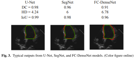
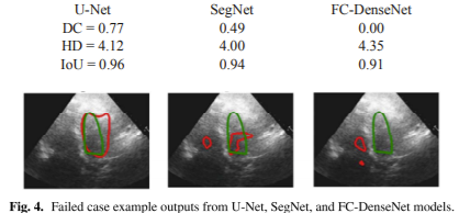
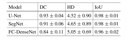
Table 1. Comparison of evaluation measures of (DC), (HD), and (IoU) between the three examine models
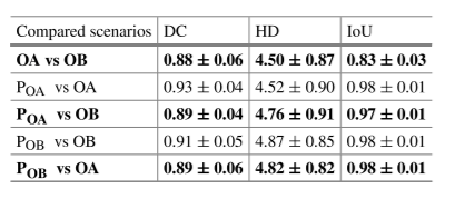
Table 2. Comparison of evaluation measures (DC), (HD), and (IoU) for the U-Net model between five possible scenarios
Table 1 provides the average Dice coefficient, Hausdorff distance, and Intersectionover-Union for the three models, across all testing images (199 images).
The U-Net model, in comparison with the SegNet and FC-DenseNet models, achieved relatively
better performance. The average Hausdorff distance, however, was higher for the FCDenseNet, compared to the other two models.
For each image, there were four assessments of the LV border; two human and two
automated (trained by the annotation of either of human operators). As shown in Table 2,
the automated models perform similarly to human operators.
The automated model
disagrees with the Operator-A, but so does the Operator-B. Since different experts make
different judgments, it is not possible for any automated model to agree with all experts.
However, it is desirable for the automated models do not have larger discrepancies when
compared with the performance of human judgments; that is, to behave approximately
as well as human operators.
Conclusion and Future Work
The time-consuming and operator-dependent process of manual annotation of left ventricle border on a 2D echocardiographic recording could be assisted by the automated
models that do not require human intervention. Our study investigated the feasibility of
such automated models which perform no worse than human experts.
The automated models demonstrate larger discrepancies with the gold-standard
annotations when encountered with the lower image qualities. This is potentially caused
by the lack of balanced data in terms of different image quality levels. Since the patient
data in our study was obtained by the expert echocardiographers, the distribution leans
more towards higher average and higher quality images. This may result in the model
forming a bias towards the more condensed quality-level images. Future investigations
will examine the correlation between the performance of the deep learning model and
the image qualities, as well as using more balanced datasets.
The patients were a convenience sample drawn from those attending a cardiology
outpatient clinic. They, therefore, may not be representative of patients who enter trials
with particular enrolment criteria or of inpatients or the general population. A further
investigation will look at a wide range of subjects in any cardiovascular disease setting.
The segmentation of other cardiac views, and using data acquired by various ultrasound
vendors can also be considered for a comprehensive examination of the deep learning
models in echocardiography.